Using SQL to Query Data

An introduction to using SQL for querying data in relational databases, working with a single table

Before you read this, and if you have not used SQL in the past, I recommend you start with this post:

An Introduction to Relational Databases

We are going to use SQL Fiddle to get an initial sense of how SQL works. This is an online IDE where we can create and query a database.

Creating a Schema

Copy the following code in the left panel on SQL Fiddle, and click the “Build Schema” button. This will create a small table that we can query on the right-hand side.

CREATE TABLE IF NOT EXISTS `customers` (
  `customer_id` int(6) NOT NULL,
  `name` text  NOT NULL,
  `email` text  NOT NULL,
  `city` text NOT NULL,
  `num_products` numeric NOT NULL,
  PRIMARY KEY (`customer_id`)
 ) ;
 
  INSERT INTO `customers` (`customer_id`,`name`,`email`
                           ,`city`,`num_products`) VALUES
 (1234,'John Doe','john@email.com','Toronto',12),
 (2345,'Jane Smith','jane@email.com','Toronto',5),
 (5678,'Sam Johnson', 'sam@email.com','Ottawa',6),
 (9876, 'Magnum PI', 'mag@email.com','Vancouver', 8),
 (4388, 'Alex Kim', 'alex@email.com','London', 3);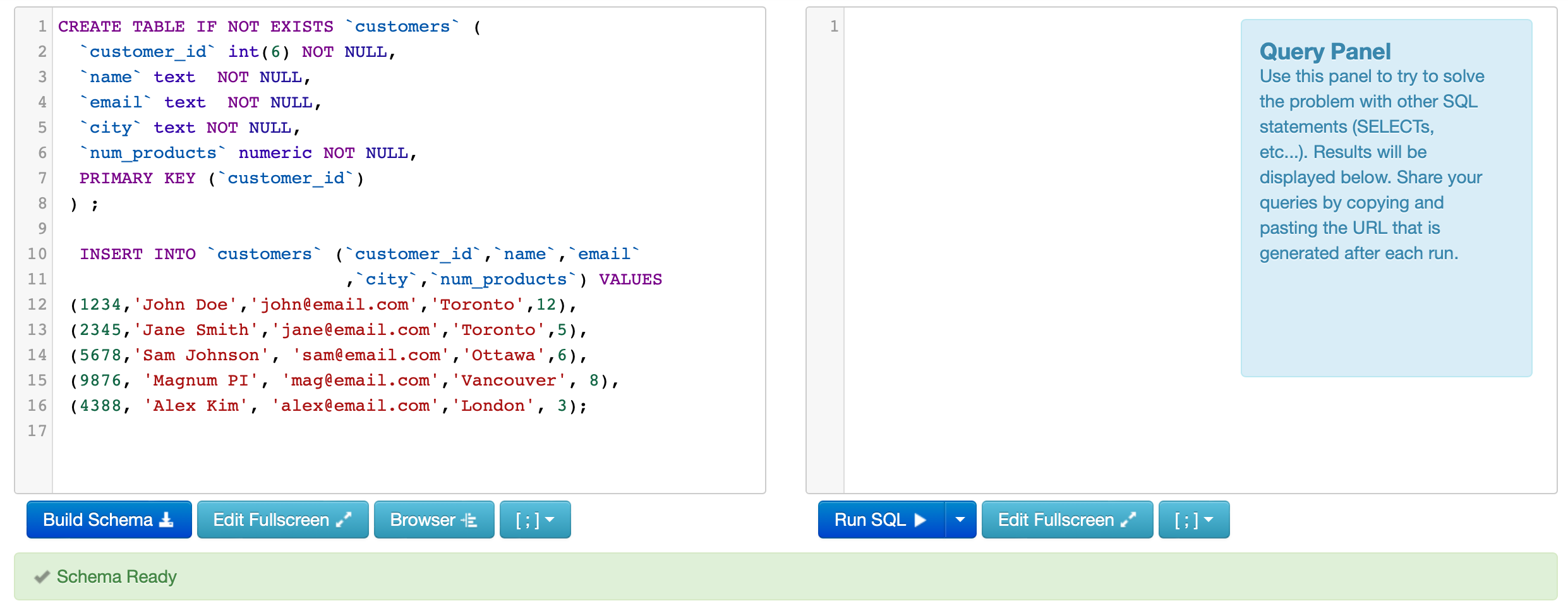

Breaking Down the Code

SQL queries generally start off with a declarative statement. For example, “CREATE” or “INSERT”. When we are creating a net new schema, we need to consider the following:

• What tables are we going to have? In this example, we are just creating a single table.

• What fields will the table have?

• What data type should each field be?

• Are there any constraints?

• Which field should be the primary key?

In the first part of our statement, we are simply creating an empty table. The statement CREATE TABLE IF NOT EXISTS allows us to create a new table while checking that this table does not already exist in the schema. We don’t want to have duplicate tables, so this is a form of control to ensure data integrity. Immediately after this statement, we give a name to our table. In this case, we have called this table `customers` and in the brackets, we are specifying the column names and conditions for each column. The first column is `customer_id` and we have set the datatype of this column to be an `int(6)` (or integer) with a maximum of 6 characters. We have also specified that this column cannot be empty with the NOT NULL statement. This means that when we insert new entries into the table, there must always be a customer_id value, otherwise the ingestion process will fail. This is another example of creating a data quality control.

The second column we created is the `name` column, which is a text field with no character limit, and it also must be NOT NULL. The `email` and `city` columns have the same conditions as the `name` column. Finally, the `num_products` column is `numeric` and also NOT NULL.

After defining the columns of our table, we have set the PRIMARY KEY(`customer_id`) which means that the `customer_id` column will be the unique identifier and primary key of this table.

To summarize, the general syntax of creating a new table in a schema is:

CREATE TABLE IF NOT EXISTS `table_name` (
`column_1` datatype NOT NULL,
`column_2` datatype NOT NULL,
PRIMARY KEY(`column_1`)
);

There are also other conditions in addition to the data type and NULL status, but we will cover those in a later module.

You will also notice that there is a semi-colon (;) placed after the statement; this signals the end of the statement. We must always identify the end, as we will need to run a new query immediately after.

The second component of our query is the INSERT INTO statement which we use to add new entries into an existing table. We specify that we will be inserting entries into the `customers` table and specifically into all three columns: (`customer_id`,`name`,`email`,`city`,`num_products`). The VALUES which will be inserted are full observations, each wrapped in a set of brackets and separated by a comma. Within the brackets, we are adding a customer identifier value (integer), a name (text), an email (text), a city (text) and a number of products (numeric). Once finished, we denote the end of the query with a semi-colon.

Now that we have created a basic table, we can click “Build Schema”, and then move on to the right hand of the screen to query the schema.

How to Query a Table with SQL

When we are writing SQL queries, we first need to consider what data we need for analysis. Let’s say we need all customer information, including the customer ID, their name and email. We can write a basic SQL query which selects all data available from a single table.

SELECT * FROM customers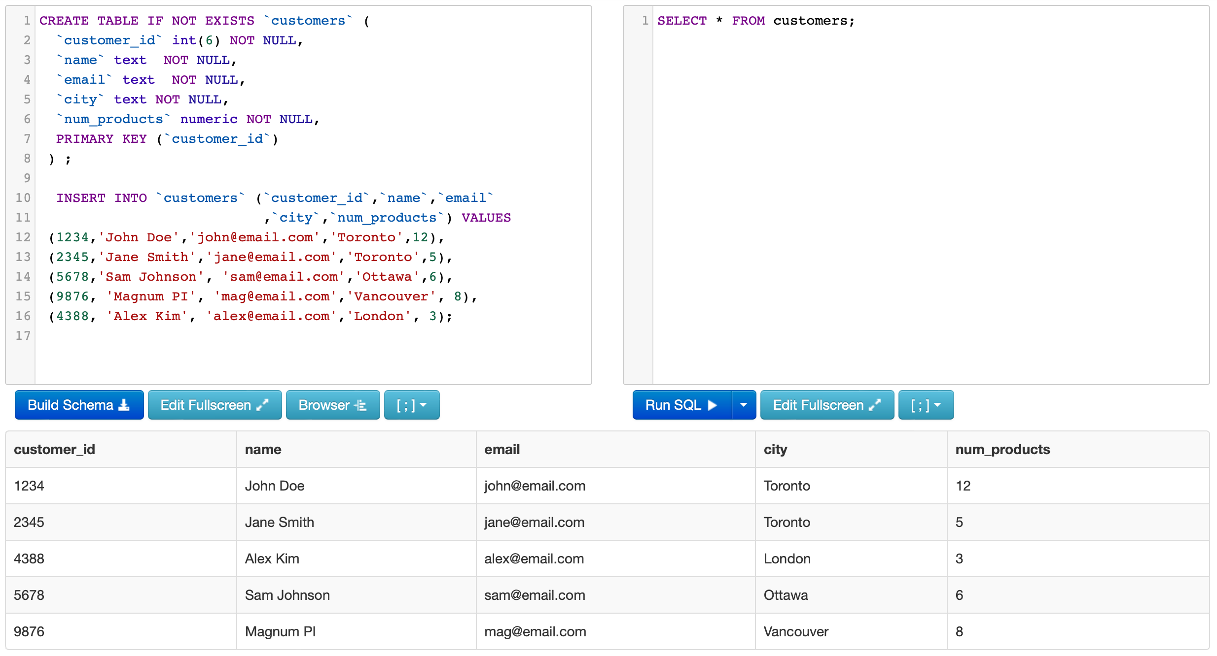

Writing this statement in the right panel of our SQL Fiddle screen will return a full table with the data we just created.

You will notice that the output lives below the two panels, and the data is organized in a tabular (or structured) format.

Breaking Down the Code

The SELECT statement declares that we are going to be pulling existing data from a table. In this case, the * symbol means that we are pulling all available columns. The FROM table determines which table we are pulling data from, and the customers part of the statement is the name of the table. This is the most basic query we can write. From here, we will continue to build on this technique.

How to Select a Specific Column with SQL

Suppose we only wanted to return customer emails. We can adjust our query slightly, by replacing the * with the specific column name we want.

SELECT email FROM customers;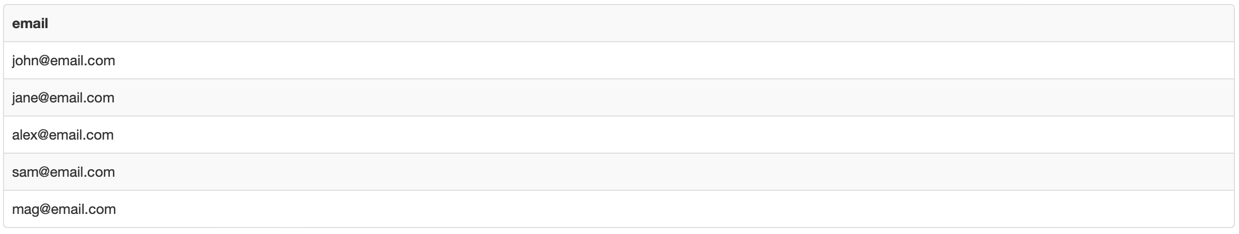

We can also select more than one column:

SELECT name, email FROM customers;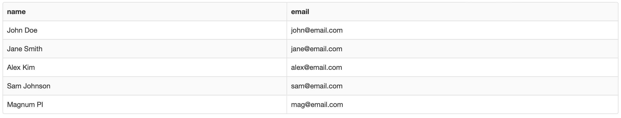

How to Add Conditions to a SQL Query

If you have worked with data in the past, it’s likely that you tend to filter or slice data in different ways. Conditions are parameters we set to filter data. In SQL, we can use a number of conditions, including:

• Exact matches

• Partial matches

• Ranges

• Greater or less than

• Multiple conditions

Let’s start by identifying the names of all customers who live in Toronto.

SELECT name FROM customers WHERE city = 'Toronto';

This query returns two names. You will notice that since we only select the name field, we receive no other information. The filtering happens in the background.

We use the WHERE statement to specify filters. This statement always comes after the FROM statement. We do not need to include the filtered column in the output, but we can if we want to. Our statement will be adjusted slightly to:

SELECT city, name FROM customers WHERE city = 'Toronto';

Now suppose we wanted to find customers who live in Toronto with more than 5 products. We can add multiple conditions using the ADD statement:

SELECT city, name, num_products FROM customers WHERE city = 'Toronto' AND num_products > 5;

This query should return only John Doe’s record. In addition to AND, we can use OR and BETWEEN statements. For example, let’s find the customers who live in Toronto or Ottawa:

SELECT city, name FROM customers WHERE city = 'Toronto' OR city = 'Ottawa';

This query will return 3 records. Now let’s find customers who have between 2 and 10 products:

SELECT city, name, num_products FROM customers WHERE num_products BETWEEN 2 AND 10;

We can also combine conditional combinations. Let’s find customers who live in Toronto or Ottawa and have more than 2 products:

SELECT city, name, num_products FROM customers WHERE (city = 'Toronto' OR city = 'Ottawa') AND num_products > 2;

You will notice I added brackets around the city condition. This is because the AND statement combines conditions together, but the OR statement begins to look for something new. Without the brackets, SQL will interpret this as looking for all customers in Toronto OR customers in Ottawa with more than 2 products. We can use brackets in any part of the statement to set the order of operations. Finally, if you have a condition which applies to the same column, you can use the IN statement:

SELECT city, name, num_products FROM customers WHERE city IN ('Toronto','Ottawa') AND num_products > 2;

Both queries will return the same result.

Let’s look at partial matches next. Suppose you wanted to find all customers whose names begin with the letter “S”. We can use the wildcard symbol %, which is in fact the percentage symbol (also called a modulo), to specify ‘any match’. For example, if we want customers whose names start with the letter “S”, we need to use the LIKE parameter:

SELECT name, city FROM customers WHERE name LIKE 'S%';

What about people whose name ends with the letter “h”?

SELECT name, city FROM customers WHERE name LIKE '%h';

We use the modulo to replace any part of a string (or text data point) which we do not know. We can also place a module on either side of a term if we don’t know what comes before or after the partial match. Let’s find people with the letter “m” anywhere in their name:

SELECT name, city FROM customers WHERE name LIKE '%m%';

How to Sort Data in SQL

By now we know how to select specific columns, and how to filter data. Another common function of data manipulation is sorting data. In SQL, we can use the ORDER BY command, along with ASC and DESC to sort data. This will come after the WHERE statement. Let’s organize our table by name:

SELECT name, city FROM customers ORDER BY name;

The default ordering methodology is ASC (or ascending order); you could specify this, but it is not necessary if you want to order from smallest to largest (or in alphabetical order). If you would like reverse order, you do need to specify the ‘descending’ parameter DESC:

SELECT name, city FROM customers ORDER BY name DESC;

Let’s add a condition:

SELECT name, city FROM customers WHERE city = 'Toronto' ORDER BY name DESC;

How to Aggregate Data in SQL

The analyses we have done so far have largely focused on working with individual records. But often, our analytical questions go a step further - perhaps we want to know the average number of products for customers in Toronto.

Whenever we use summary statistics in analysis, this is called aggregation. In programming, there are various functions we can use to aggregate data. If you’ve used MS Excel in the past, you may have done this with a pivot table.

SQL offers the following aggregation functions:

COUNT
SUM
AVG
MIN
MAX
VAR
STDEV

We can apply these functions to an entire table, or we can create sub-segments of data using a GROUP BY statement. Let’s look at an entire table first. Let’s count the number of customers:

SELECT COUNT(name) FROM customers;

This query should return the value of 5. We can also count unique values using the DISTINCT parameter. Let’s count the number of unique cities we have in our dataset:

SELECT COUNT(DISTINCT city) FROM customers;

This query should return the value of 4. Now let’s add up the total number of products our customers have:

SELECT SUM(num_products) FROM customers;

This query should return 34 total products. We can also add multiple aggregation statements. Let’s look at both the total and average number of products in the data set:

SELECT SUM(num_products), AVG(num_products) FROM customers;

Our output should consist of two columns with the total of 34 and the average of 6.8 products.

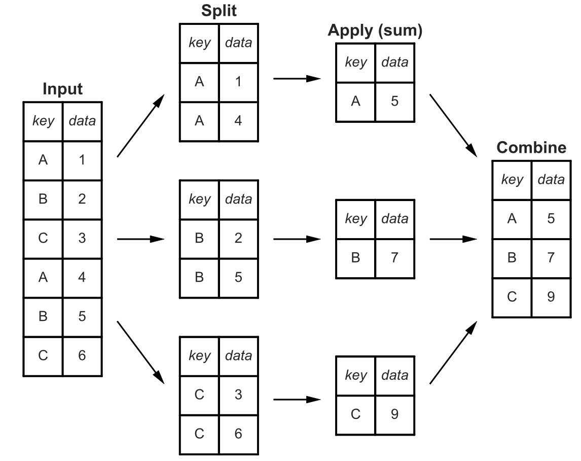
This is a great start, but we may want to dive deeper into the analysis and segment data in a meaningful way. For example, suppose we wanted to calculate the total and average number of products by city. We can use the GROUP BY statement to do this. But first, how does GROUP BY work? It essentially identifies all repeated rows and values, then applies an aggregation, and combines aggregated data back into a table.

The GROUP BY statement always comes after the FROM statement. Let’s find the total and average number of products by city:

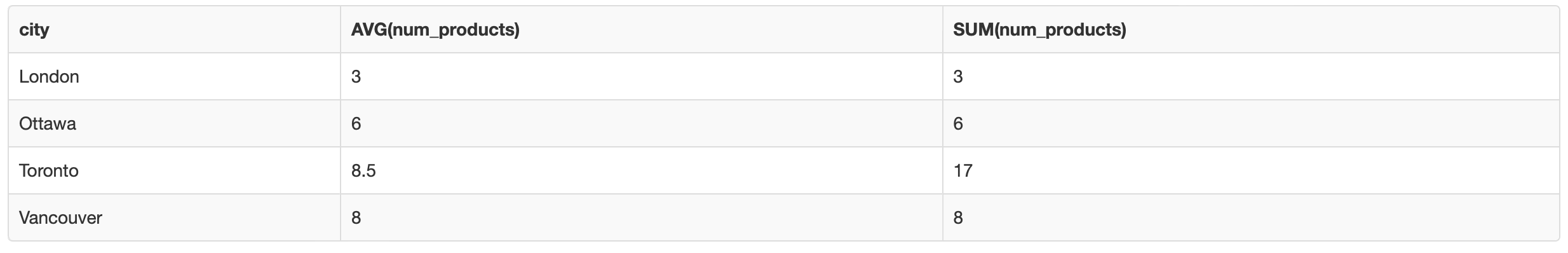
SELECT city, AVG(num_products), SUM(num_products) FROM customers GROUP BY city;

Your output should be a 3-column table which provides summary statistics by city:

Adding Conditions to a GROUP BY Statement in SQL

There are two options when filtering data which is grouped. We can use the WHERE statement to filter before the GROUP BY statement; or we can use the HAVING statement to filter the table after the GROUP BY statement. Let’s look at an example of each:

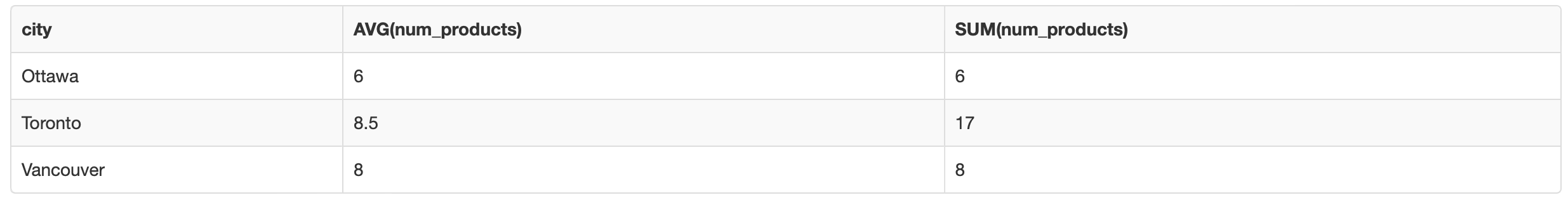
SELECT city, AVG(num_products), SUM(num_products) FROM customers WHERE city = 'Toronto' OR city = 'Ottawa' GROUP BY city;

This query will return the following output:

Alternatively, we can use HAVING:

SELECT city, AVG(num_products), SUM(num_products) FROM customers GROUP BY city HAVING city = 'Toronto' OR city = 'Ottawa';

The output is the same! When we are filtering using HAVING, we need to filter the grouped table. Note that some column names may have changed - for example, the grouped table has new columns called “AVG(num_products)” and “SUM(num_products)”, where as the original table has a column called “num_products”.

Suppose we wanted to only aggregate customers who had more than 2 products - this filter would need to come BEFORE the aggregation, thus we would have:

SELECT city, AVG(num_products), SUM(num_products) FROM customers WHERE num_products > 2 GROUP BY city;

Our output would be:

Suppose instead we wanted cities where the average number of products was greater than 5 - in this case, we would need to filter the grouped object:

SELECT city, AVG(num_products), SUM(num_products) FROM customers GROUP BY city HAVING AVG(num_products) > 5;

Now our output looks like this:

Note: we also changed the column name when using HAVING from “num_products” to “AVG(num_products)”.

Bringing it All Together

Finally, let’s write one query which aggregates, groups, filters and orders data:

SELECT city, AVG(num_products), SUM(num_products) FROM customers GROUP BY city HAVING AVG(num_products) > 2 ORDER BY city DESC;

And an example with WHERE:

SELECT city, AVG(num_products), SUM(num_products) FROM customers WHERE city IN ('Toronto','Ottawa') AND num_products > 2 GROUP BY city ORDER BY SUM(num_products) DESC;

Congratulations! You now know the basics of writing SQL queries.